Note: This calculation does not support jax. [jan25]

[1]:

%matplotlib inline
import matplotlib.pyplot as plt
plt.rcParams.update({
    "text.usetex": True,
    "font.family": "sans-serif",
    "font.sans-serif": "Helvetica",
})
import numpy as np
import os
from classy_sz import Class as Class_sz

[2]:

import classy_szfast

Cosmological parameters

[3]:

cosmo_params= {
# 'omega_b': 0.02242,
# 'omega_cdm':  0.11933,
# 'H0': 67.66,
# 'tau_reio': 0.0561,
# 'ln10^{10}A_s': 3.047,
# 'n_s': 0.9665,
# "cosmo_model": 0, # use 0: lcdm, 1: mnu-lcdm emulators


    'omega_b': 0.02,
    'omega_cdm':  0.12,
    'H0': 80.,
    'tau_reio': 0.0561,
    'ln10^{10}A_s': 3.047,
    'n_s': 0.9665,
    "cosmo_model": 0, # 1: use mnu-lcdm emulators; 0: use lcdm with fixed neutrino mass

    # "ell_min" : 2,
    # "ell_max" : 8000,

    # 'dlogell': 0.2,
    # 'z_min' : 0.005,
    # 'z_max' : 3.0,
    # 'M_min' : 1.0e10,
    # 'M_max' : 3.5e15,

    # "P0GNFW": 8.130,
    # "c500": 1.156,
    # "gammaGNFW": 0.3292,
    # "alphaGNFW": 1.0620,
    # "betaGNFW":5.4807,
    "B": 1.2,
    # "jax": 1,
}

Precision parameters

[7]:

precision_params = {
'x_outSZ': 4., # truncate profile beyond x_outSZ*r_s

'n_m_pressure_profile' :10, # default: 100, decrease for faster
'n_z_pressure_profile' :10, # default: 100, decrease for faster


'use_fft_for_profiles_transform' : 1, # use fft's or not.
# only used if use_fft_for_profiles_transform set to 1
'N_samp_fftw' :1024,
'x_min_gas_pressure_fftw' : 1e-4,
'x_max_gas_pressure_fftw' : 1e6,


'ndim_redshifts' :150,


'redshift_epsabs': 1.0e-40,
'redshift_epsrel': 0.0001,


'mass_epsabs': 1.0e-40,
'mass_epsrel': 0.0001
}

Generalized NFW pressure profile

[8]:

%%time

classy_sz = Class_sz()
classy_sz.set(cosmo_params)
classy_sz.set(precision_params)
classy_sz.set({

'output': 'tSZ_tSZ_1h,tSZ_tSZ_2h',
'skip_input':0,
"ell_min" : 2,
"ell_max" : 8000,
'dell': 0.,
'dlogell': 0.2,

'z_min' : 0.005,
'z_max' : 3.0,
'M_min' : 5e10,
'M_max' : 3.5e15,


'mass_function' : 'T08M500c',



'pressure_profile':'GNFW', # can be Battaglia, Arnaud, etc

"P0GNFW": 8.130,
"c500": 1.156,
"gammaGNFW": 0.3292,
"alphaGNFW": 1.0620,
"betaGNFW":5.4807,

"cosmo_model": 0, # lcdm

'no_spline_in_tinker': 1,
'HMF_prescription_NCDM': 1,


})
classy_sz.initialize_classy_szfast()

CPU times: user 882 ms, sys: 6.29 ms, total: 888 ms
Wall time: 191 ms

[9]:

# classy_sz.pars
%timeit -n 10 classy_sz.initialize_classy_szfast()

105 ms ± 2.26 ms per loop (mean ± std. dev. of 7 runs, 10 loops each)

[10]:

l = np.asarray(classy_sz.cl_sz()['ell'])
cl_yy_1h = np.asarray(classy_sz.cl_sz()['1h'])
cl_yy_2h = np.asarray(classy_sz.cl_sz()['2h'])

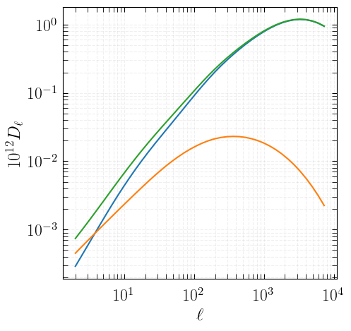
[11]:

label_size = 17
title_size = 18
legend_size = 13
handle_length = 1.5
fig, (ax1) = plt.subplots(1,1,figsize=(5,5))
ax = ax1
ax.tick_params(axis = 'x',which='both',length=5,direction='in', pad=10)
ax.tick_params(axis = 'y',which='both',length=5,direction='in', pad=5)
ax.xaxis.set_ticks_position('both')
ax.yaxis.set_ticks_position('both')
plt.setp(ax.get_yticklabels(), rotation='horizontal', fontsize=label_size)
plt.setp(ax.get_xticklabels(), fontsize=label_size)
ax.grid( visible=True, which="both", alpha=0.2, linestyle='--')
ax.set_xlabel(r"$\ell$ ",size=title_size)
ax.set_ylabel(r"$10^{12}D_\ell$",size=title_size)
ax.set_xscale('log')
ax.set_yscale('log')

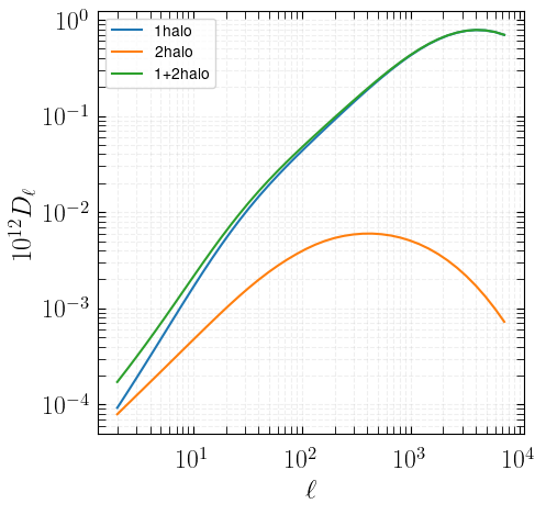
ax.plot(l,cl_yy_1h,label='1halo')
ax.plot(l,cl_yy_2h,label='2halo')
ax.plot(l,cl_yy_2h+cl_yy_1h,label='1+2halo')
ax.legend()

[11]:

<matplotlib.legend.Legend at 0x16357f410>

[12]:

classy_sz.get_gas_profile_at_x_M_z_nfw_200c(0.1,1e14,0.2)

[12]:

2404242162572997.5

[13]:

dndlnm = np.vectorize(classy_sz.get_dndlnM_at_z_and_M)

[14]:

classy_sz.Rho_crit_0()#,277517901355.06506

[14]:

277517901355.06506

[9]:

allpars = {
    'omega_b': 0.02,
    'omega_cdm':  0.12,
    'H0': 80.,
    'tau_reio': 0.0561,
    'ln10^{10}A_s': 3.047,
    'n_s': 0.9665,
    "cosmo_model": 0, # 1: use mnu-lcdm emulators; 0: use lcdm with fixed neutrino mass

    "ell_min" : 2,
    "ell_max" : 8000,

    'dlogell': 0.2,
    'z_min' : 0.005,
    'z_max' : 3.0,
    'M_min' : 1.0e10,
    'M_max' : 3.5e15,

    "P0GNFW": 8.130,
    "c500": 1.156,
    "gammaGNFW": 0.3292,
    "alphaGNFW": 1.0620,
    "betaGNFW":5.4807,
    "B": 1.2,
    # "jax": 1,
}

params_values_dict = allpars
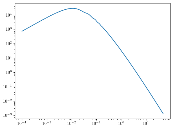
pks, ks = classy_sz.get_pkl_at_z(zp, params_values_dict= params_values_dict)
plt.loglog(ks,pks)

[9]:

[<matplotlib.lines.Line2D at 0x3cfb3aff0>]

[10]:

pks[0]

[10]:

array([725.34335548])

Arnaud et al 2010 tabulated profile

[23]:

%%time
classy_sz_A10 = Class_sz()
classy_sz_A10.set(cosmo_params)
classy_sz_A10.set(precision_params)
classy_sz_A10.set({

'output': 'tSZ_1h,tSZ_2h',

"ell_min" : 2,
"ell_max" : 8000,
'dell': 0,
'dlogell': 0.2,

'z_min' : 0.005,
'z_max' : 3.0,
'M_min' : 1.0e10,
'M_max' : 3.5e15,


'mass_function' : 'T08M500c',

'pressure_profile':'A10', # can be Battaglia, Arnaud, etc

'cosmo_model': 0,

})
classy_sz_A10.initialize_classy_szfast()

CPU times: user 3.31 s, sys: 545 ms, total: 3.85 s
Wall time: 487 ms

[24]:

l_A10 = np.asarray(classy_sz_A10.cl_sz()['ell'])
cl_yy_1h_A10 = np.asarray(classy_sz_A10.cl_sz()['1h'])
cl_yy_2h_A10 = np.asarray(classy_sz_A10.cl_sz()['2h'])

[25]:

label_size = 17
title_size = 18
legend_size = 13
handle_length = 1.5
fig, (ax1) = plt.subplots(1,1,figsize=(5,5))
ax = ax1
ax.tick_params(axis = 'x',which='both',length=5,direction='in', pad=10)
ax.tick_params(axis = 'y',which='both',length=5,direction='in', pad=5)
ax.xaxis.set_ticks_position('both')
ax.yaxis.set_ticks_position('both')
plt.setp(ax.get_yticklabels(), rotation='horizontal', fontsize=label_size)
plt.setp(ax.get_xticklabels(), fontsize=label_size)
ax.grid( visible=True, which="both", alpha=0.2, linestyle='--')
ax.set_xlabel(r"$\ell$ ",size=title_size)
ax.set_ylabel(r"$10^{12}D_\ell$",size=title_size)
ax.set_xscale('log')
ax.set_yscale('log')

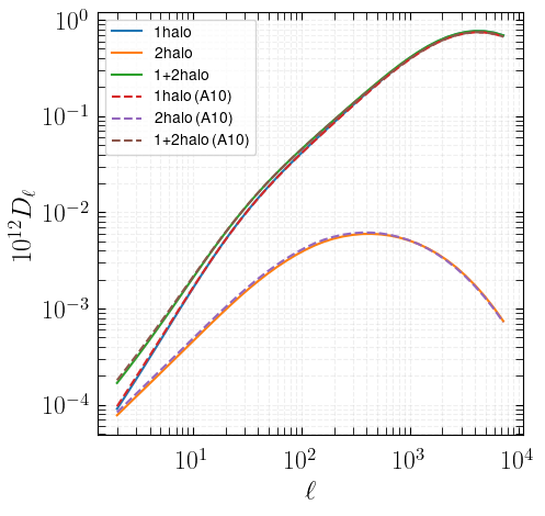
ax.plot(l,cl_yy_1h,label='1halo')
ax.plot(l,cl_yy_2h,label='2halo')
ax.plot(l,cl_yy_2h+cl_yy_1h,label='1+2halo')

ax.plot(l_A10,cl_yy_1h_A10,label='1halo (A10)',ls='--')
ax.plot(l_A10,cl_yy_2h_A10,label='2halo (A10)',ls='--')
ax.plot(l_A10,cl_yy_2h_A10+cl_yy_1h_A10,label='1+2halo (A10)',ls='--')
ax.legend()

[25]:

<matplotlib.legend.Legend at 0x3570b7680>

Planck 2013 tabulated profile

[6]:

%%time
classy_sz_P13 = Class_sz()
classy_sz_P13.set(cosmo_params)
classy_sz_P13.set(precision_params)
classy_sz_P13.set({

'output': 'tSZ_1h,tSZ_2h',

"ell_min" : 2,
"ell_max" : 8000,
'dell': 0,
'dlogell': 0.2,

'z_min' : 0.005,
'z_max' : 3.0,
'M_min' : 1.0e10,
'M_max' : 3.5e15,


'mass_function' : 'T08M500c',

'pressure_profile':'P13', # can be Battaglia, Arnaud, etc

'cosmo_model': 0,

})
classy_sz_P13.compute_class_szfast()

CPU times: user 3.06 s, sys: 472 ms, total: 3.53 s
Wall time: 471 ms

[9]:

l_P13 = np.asarray(classy_sz_P13.cl_sz()['ell'])
cl_yy_1h_P13 = np.asarray(classy_sz_P13.cl_sz()['1h'])
cl_yy_2h_P13 = np.asarray(classy_sz_P13.cl_sz()['2h'])

[10]:

label_size = 17
title_size = 18
legend_size = 13
handle_length = 1.5
fig, (ax1) = plt.subplots(1,1,figsize=(5,5))
ax = ax1
ax.tick_params(axis = 'x',which='both',length=5,direction='in', pad=10)
ax.tick_params(axis = 'y',which='both',length=5,direction='in', pad=5)
ax.xaxis.set_ticks_position('both')
ax.yaxis.set_ticks_position('both')
plt.setp(ax.get_yticklabels(), rotation='horizontal', fontsize=label_size)
plt.setp(ax.get_xticklabels(), fontsize=label_size)
ax.grid( visible=True, which="both", alpha=0.2, linestyle='--')
ax.set_xlabel(r"$\ell$ ",size=title_size)
ax.set_ylabel(r"$10^{12}D_\ell$",size=title_size)
ax.set_xscale('log')
ax.set_yscale('log')


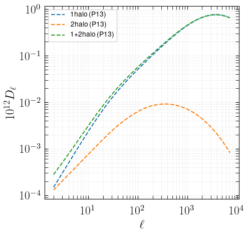
ax.plot(l_P13,cl_yy_1h_P13,label='1halo (P13)',ls='--')
ax.plot(l_P13,cl_yy_2h_P13,label='2halo (P13)',ls='--')
ax.plot(l_P13,cl_yy_2h_P13+cl_yy_1h_P13,label='1+2halo (P13)',ls='--')
ax.legend()

[10]:

<matplotlib.legend.Legend at 0x3523f6e10>

Battaglia et al 2012 pressure profile

[32]:

%%time
classy_sz = Class_sz()
classy_sz.set(cosmo_params)
classy_sz.set(precision_params)
classy_sz.set({

'output': 'tSZ_1h,tSZ_2h',

"ell_min" : 2,
"ell_max" : 8000,
'dell': 0,
'dlogell': 0.2,

'z_min' : 0.005,
'z_max' : 3.0,
'M_min' : 1.0e10,
'M_max' : 3.5e15,


'mass_function' : 'T08M200c',

'pressure_profile':'B12', # can be Battaglia, Arnaud, etc
'concentration_parameter':"D08",

})
classy_sz.compute_class_szfast()

CPU times: user 10.3 s, sys: 1.97 s, total: 12.3 s
Wall time: 1.61 s

[33]:

l = np.asarray(classy_sz.cl_sz()['ell'])
cl_yy_1h = np.asarray(classy_sz.cl_sz()['1h'])
cl_yy_2h = np.asarray(classy_sz.cl_sz()['2h'])

[34]:

label_size = 17
title_size = 18
legend_size = 13
handle_length = 1.5
fig, (ax1) = plt.subplots(1,1,figsize=(5,5))
ax = ax1
ax.tick_params(axis = 'x',which='both',length=5,direction='in', pad=10)
ax.tick_params(axis = 'y',which='both',length=5,direction='in', pad=5)
ax.xaxis.set_ticks_position('both')
ax.yaxis.set_ticks_position('both')
plt.setp(ax.get_yticklabels(), rotation='horizontal', fontsize=label_size)
plt.setp(ax.get_xticklabels(), fontsize=label_size)
ax.grid( visible=True, which="both", alpha=0.2, linestyle='--')
ax.set_xlabel(r"$\ell$ ",size=title_size)
ax.set_ylabel(r"$10^{12}D_\ell$",size=title_size)
ax.set_xscale('log')
ax.set_yscale('log')

ax.plot(l,cl_yy_1h,label='1halo')
ax.plot(l,cl_yy_2h,label='2halo')
ax.plot(l,cl_yy_2h+cl_yy_1h,label='1+2halo')

[34]:

[<matplotlib.lines.Line2D at 0x407a4e7b0>]

Trispectrum and Covariance Matrix Calculation

Set sky-fraction:

[13]:

fsky = 1.

Multipole range:

[14]:

ell_min = 100
ell_max = 8000
dlogell = 0.2

[15]:

%%time
classy_sz = Class_sz()
classy_sz.set(cosmo_params)
classy_sz.set(precision_params)
classy_sz.set({

'output': 'tSZ_1h,tSZ_Trispectrum',

"ell_min" : ell_min,
"ell_max" : ell_max,
'dell': 0.,
'dlogell': dlogell,

# 'z_min' : 0.005,
'z_max' : 3.0,
'M_min' : 1.0e10,
'M_max' : 3.5e15,


'mass_function' : 'T08M500c',
'pressure_profile':'A10',


})
classy_sz.compute_class_szfast()

CPU times: user 10.7 s, sys: 1.37 s, total: 12.1 s
Wall time: 1.61 s

Determine number fo modes in each bins:

[16]:

l = np.asarray(classy_sz.cl_sz()['ell'])

[17]:

[17]:

array([ 100.        ,  122.14027582,  149.18246976,  182.21188004,
        222.55409285,  271.82818285,  332.01169227,  405.51999668,
        495.30324244,  604.96474644,  738.90560989,  902.50134994,
       1102.31763806, 1346.3738035 , 1644.46467711, 2008.55369232,
       2453.25301971, 2996.41000474, 3659.82344437, 4470.11844933,
       5459.81500331, 6668.63310409])

[18]:

bin_edges = np.sqrt(l[:-1] * l[1:])
bin_edges = np.concatenate(([ell_min], bin_edges, [ell_max]))

[19]:

all_ls = np.arange(ell_min,ell_max)

[20]:

dells , _ = np.histogram(all_ls, bins=bin_edges)

[21]:

%%time


dl_yy_1h = np.asarray(classy_sz.cl_sz()['1h'])
tllprime_sz = classy_sz.tllprime_sz().copy() # note: sqrt(T_ll') ~ 10^12 y^2 ~ C_l
tllp = np.zeros((len(l),len(l)))
mllp = np.zeros((len(l),len(l)))
mllpG = np.zeros((len(l),len(l)))
for il in range(len(l)):
    for ilp in range(len(l)):
        lil =l[il]
        lilp = l[ilp]
        dell = dells[il]
        sig_gauss_l = np.sqrt(2./(2*lil+1.))*dl_yy_1h[il]/np.sqrt(dell*fsky)
        if il == ilp:
            mllp[il][ilp] = (sig_gauss_l*sig_gauss_l+lil*(lil+1.)/2./np.pi*lilp*(lilp+1.)/2./np.pi*tllprime_sz[il][ilp]/4./np.pi/fsky)*1e-24
            mllpG[il][ilp] = (sig_gauss_l*sig_gauss_l)*1e-24
        else:
            mllp[il][ilp] = lil*(lil+1.)/2./np.pi*lilp*(lilp+1.)/2./np.pi*tllprime_sz[il][ilp]/4./np.pi/fsky*1e-24
        tllp[il][ilp] = lil*(lil+1.)/2./np.pi*lilp*(lilp+1.)/2./np.pi*tllprime_sz[il][ilp]*1e-24

CPU times: user 5.24 ms, sys: 333 μs, total: 5.58 ms
Wall time: 6.17 ms

[22]:

plt.imshow(tllp)
plt.title("class_sz")
plt.colorbar()

[22]:

<matplotlib.colorbar.Colorbar at 0x4211d2cc0>

../_images/notebooks_class_sz_tszpowerspectrum_42_1.png

[23]:

label_size = 17
title_size = 18
legend_size = 13
handle_length = 1.5
fig, (ax1) = plt.subplots(1,1,figsize=(5,5))
ax = ax1
ax.tick_params(axis = 'x',which='both',length=5,direction='in', pad=10)
ax.tick_params(axis = 'y',which='both',length=5,direction='in', pad=5)
ax.xaxis.set_ticks_position('both')
ax.yaxis.set_ticks_position('both')
plt.setp(ax.get_yticklabels(), rotation='horizontal', fontsize=label_size)
plt.setp(ax.get_xticklabels(), fontsize=label_size)
ax.grid( visible=True, which="both", alpha=0.2, linestyle='--')
ax.set_xlabel(r"$\ell$ ",size=title_size)
ax.set_ylabel(r"$10^{12}D_\ell$",size=title_size)
ax.set_xscale('log')
ax.set_yscale('log')

ax.plot(l,dl_yy_1h,label='1halo',marker='o',markersize=2.,lw=0.1)
for edge in bin_edges:
    ax.axvline(edge, color='red', linestyle='--', linewidth=0.7,alpha=0.2)  # Customize as needed

yerrG = np.sqrt(np.diag(mllpG))
yerrTOT = np.sqrt(np.diag(mllp))
ax.errorbar(l,dl_yy_1h,yerr=1e12*yerrTOT,ls='None',c='k')
ax.errorbar(l,dl_yy_1h,yerr=1e12*yerrG,ls='None',c='r')
ax.set_xlim(100,10000)

[23]:

(100, 10000)

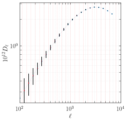
../_images/notebooks_class_sz_tszpowerspectrum_43_1.png

Note that the Gaussian contribution in first bin here only accounts for half the number of modes. Either truncate it, or ammend the code above.

Mass and redshift dependence of integrand

[24]:

%matplotlib inline
import matplotlib
import matplotlib.pyplot as plt
plt.rcParams.update({
    "text.usetex": True,
    "font.family": "sans-serif",
    "font.sans-serif": "Helvetica",
})
import numpy as np
import os
from classy_sz import Class as Class_sz

[25]:

cosmo_params= {
'omega_b': 0.02242,
'omega_cdm':  0.11933,
'H0': 67.66,
'tau_reio': 0.0561,
'ln10^{10}A_s': 3.047,
'n_s': 0.9665,
}

[26]:

precision_params = {
'x_outSZ': 4., # truncate profile beyond x_outSZ*r_s
'use_fft_for_profiles_transform' : 1, # use fft's or not.
# only used if use_fft_for_profiles_transform set to 1
'N_samp_fftw' : 512,
'x_min_gas_pressure_fftw' : 1e-4,
'x_max_gas_pressure_fftw' : 1e4,
}

[27]:

zmin = 0.001
zmax = 5.
mmin = 1e11 # msun /h
mmax = 5e15 # msun / h

[28]:

%%time

classy_sz = Class_sz()
classy_sz.set(cosmo_params)
classy_sz.set(precision_params)
classy_sz.set({

'output': 'tSZ_tSZ_1h',

"ell_min" : 2,
"ell_max" : 8000,
'dell': 0,
'dlogell': 0.2,

'z_min' : zmin,
'z_max' : zmax,
'M_min' : mmin,
'M_max' : mmax,


'mass_function' : 'T08M500c',



'pressure_profile':'custom_gnfw', # can be Battaglia, Arnaud, etc

"P0GNFW": 8.130,
"c500": 1.156,
"gammaGNFW": 0.3292,
"alphaGNFW": 1.0620,
"betaGNFW":5.4807,

"cosmo_model": 0, # lcdm with Mnu=0.06ev fixed

})
classy_sz.compute_class_szfast()

/Users/boris/venvdir/class_sz_312_brew/lib/python3.12/site-packages/mcfit/mcfit.py:130: UserWarning: use backend='jax' if desired
  warnings.warn("use backend='jax' if desired")

CPU times: user 21.8 s, sys: 2.28 s, total: 24.1 s
Wall time: 3.33 s

[29]:

l = np.asarray(classy_sz.cl_sz()['ell'])
cl_yy_1h = np.asarray(classy_sz.cl_sz()['1h'])
cl_yy_2h = np.asarray(classy_sz.cl_sz()['2h'])

[30]:

label_size = 17
title_size = 18
legend_size = 13
handle_length = 1.5
fig, (ax1) = plt.subplots(1,1,figsize=(5,5))
ax = ax1
ax.tick_params(axis = 'x',which='both',length=5,direction='in', pad=10)
ax.tick_params(axis = 'y',which='both',length=5,direction='in', pad=5)
ax.xaxis.set_ticks_position('both')
ax.yaxis.set_ticks_position('both')
plt.setp(ax.get_yticklabels(), rotation='horizontal', fontsize=label_size)
plt.setp(ax.get_xticklabels(), fontsize=label_size)
ax.grid( visible=True, which="both", alpha=0.2, linestyle='--')
ax.set_xlabel(r"$\ell$ ",size=title_size)
ax.set_ylabel(r"$D_\ell$",size=title_size)
ax.set_xscale('log')
ax.set_yscale('log')
# ax.set_ylim(1e-1,1e4)
# ax.set_xlim(5e-2,1e1)
ax.plot(l,cl_yy_1h,label='1halo')
# # plt.xlim(2e-2,4e1)
# plt.ylim(1e-2,1e4)
ax.legend()

[30]:

<matplotlib.legend.Legend at 0x3f2e0d460>

../_images/notebooks_class_sz_tszpowerspectrum_52_1.png

[31]:

%%time
dyl2dzdlnm = np.vectorize(classy_sz.get_dyl2dzdlnm_at_z_and_m)
z_array_2d = np.linspace(0.01,2.5,500)
log10m_array = np.linspace(np.log10(1e12),np.log10(1e16),500)
dyl2dzdm_2d = np.zeros((500,500))


dyl2dzdm_2d = np.transpose(dyl2dzdlnm(z_array_2d[None,:],10**log10m_array[:,None],l=500))

CPU times: user 566 ms, sys: 12.6 ms, total: 579 ms
Wall time: 613 ms

[32]:

im = plt.imshow(dyl2dzdm_2d, cmap='hot', interpolation='nearest',
                extent = [12,16,z_array_2d[-1],z_array_2d[0]],
                aspect='auto')
cbar = plt.colorbar(im) # adding the colobar on the right

plt.xlabel(r'$\mathrm{log}_{10}(m)$')
plt.ylabel(r'$z$')
# plt.show()
_ = plt.title(r'$\ell = 500$')

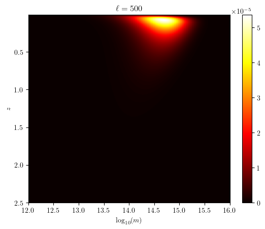
../_images/notebooks_class_sz_tszpowerspectrum_54_0.png

Note that dyl2dzdm_2d is weighted by the volume element and halo-mass function. It is the integrand of the 1-halo term of the tSZ power spectrum.

We can also take slices of the 3d plot.

[33]:

nz = 500
nm = 500
zs = np.linspace(zmin,zmax,nz)
ms = np.geomspace(mmin,mmax,nm)

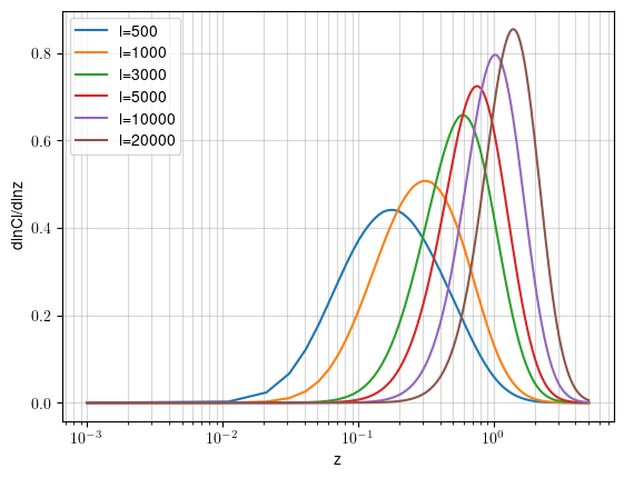
for l in [500,1000,3000,5000,10000,20000]:
    dlnCldlnz = zs*[np.trapz(dyl2dzdlnm(z,ms,l=l),x=np.log(ms)) for z in zs]
    dlnCldlnz *= 1./np.trapz(dlnCldlnz/zs,x=zs)

    plt.plot(zs,dlnCldlnz,label=f'l={l}')
plt.legend()
plt.grid(which='both',alpha=0.5)
_ = plt.xlabel('z')
_ = plt.ylabel('dlnCl/dlnz')
plt.xscale('log')

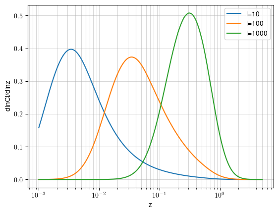
../_images/notebooks_class_sz_tszpowerspectrum_57_0.png

[34]:

nz = 500
nm = 500
zs = np.geomspace(zmin,zmax,nz)
ms = np.geomspace(mmin,mmax,nm)


for l in [10,100,1000]:
    dlnCldlnz = zs*[np.trapz(dyl2dzdlnm(z,ms,l=l),x=np.log(ms)) for z in zs]
    dlnCldlnz *= 1./np.trapz(dlnCldlnz,x=np.log(zs))

    plt.plot(zs,dlnCldlnz,label=f'l={l}')
plt.legend()
plt.grid(which='both',alpha=0.5)
_ = plt.xlabel('z')
_ = plt.ylabel('dlnCl/dlnz')
plt.xscale('log')

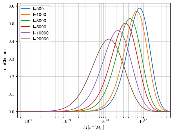
../_images/notebooks_class_sz_tszpowerspectrum_58_0.png

[35]:

for l in [500,1000,3000,5000,10000,20000]:
    dlnCldlnm = ms*[np.trapz(dyl2dzdlnm(zs,m,l=l),x=zs) for m in ms]
    dlnCldlnm *= 1./np.trapz(dlnCldlnm/ms,x=ms)

    plt.plot(ms,dlnCldlnm,label=f'l={l}')
plt.legend()
plt.grid(which='both',alpha=0.5)
_ = plt.xlabel(r'$M [h^{-1}M_\odot]$')
_ = plt.ylabel('dlnCl/dlnm')
plt.xscale('log')
_ = plt.xlim(5e11,5e15)

../_images/notebooks_class_sz_tszpowerspectrum_59_0.png

With cluster counts completeness

[1]:

%matplotlib inline
import matplotlib
import matplotlib.pyplot as plt
plt.rcParams.update({
    "text.usetex": True,
    "font.family": "sans-serif",
    "font.sans-serif": "Helvetica",
})
import numpy as np
import os
from classy_sz import Class as Class_sz

[2]:

cosmo_params= {
'omega_b': 0.02242,
'omega_cdm':  0.11933,
'H0': 67.66,
'tau_reio': 0.0561,
'ln10^{10}A_s': 3.047,
'n_s': 0.9665,
}

[3]:

precision_params = {
'x_outSZ': 4., # truncate profile beyond x_outSZ*r_s
'use_fft_for_profiles_transform' : 1, # use fft's or not.
# only used if use_fft_for_profiles_transform set to 1
# 'N_samp_fftw' : 512,
# 'x_min_gas_pressure_fftw' : 1e-4,
# 'x_max_gas_pressure_fftw' : 1e4,
}

[4]:

zmin = 0.001
zmax = 5.
mmin = 1e11 # msun /h
mmax = 5e15 # msun / h

[36]:

%%time

classy_sz = Class_sz()
classy_sz.set(cosmo_params)
classy_sz.set(precision_params)
classy_sz.set({

'output': 'tSZ_tSZ_1h',

"ell_min" : 2,
"ell_max" : 8000,
'dell': 0,
'dlogell': 0.2,

'z_min' : zmin,
'z_max' : zmax,
'M_min' : mmin,
'M_max' : mmax,


'mass_function' : 'T08M500c',



'pressure_profile':'custom_gnfw', # can be Battaglia, Arnaud, etc

"P0GNFW": 8.130,
"c500": 1.156,
"gammaGNFW": 0.3292,
"alphaGNFW": 1.0620,
"betaGNFW":5.4807,

"cosmo_model": 0, # lcdm with Mnu=0.06ev fixed


"component of tSZ power spectrum": "resolved",
"signal-to-noise_cut-off_for_survey_cluster_completeness": 6,
"y_m_relation": 0,

})
classy_sz.compute_class_szfast()
l = np.asarray(classy_sz.cl_sz()['ell'])
cl_yy_1h = np.asarray(classy_sz.cl_sz()['1h'])
cl_yy_2h = np.asarray(classy_sz.cl_sz()['2h'])


classy_sz.set({
"component of tSZ power spectrum": "unresolved",
})
classy_sz.compute_class_szfast()
cl_yy_1h_unresolved = np.asarray(classy_sz.cl_sz()['1h'])
cl_yy_2h_unresolved = np.asarray(classy_sz.cl_sz()['2h'])


classy_sz.set({
"component of tSZ power spectrum": "total",
})
classy_sz.compute_class_szfast()
cl_yy_1h_total = np.asarray(classy_sz.cl_sz()['1h'])
cl_yy_2h_total = np.asarray(classy_sz.cl_sz()['2h'])

CPU times: user 36.5 s, sys: 4.21 s, total: 40.7 s
Wall time: 5.7 s

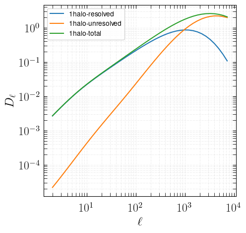
[37]:

label_size = 17
title_size = 18
legend_size = 13
handle_length = 1.5
fig, (ax1) = plt.subplots(1,1,figsize=(5,5))
ax = ax1
ax.tick_params(axis = 'x',which='both',length=5,direction='in', pad=10)
ax.tick_params(axis = 'y',which='both',length=5,direction='in', pad=5)
ax.xaxis.set_ticks_position('both')
ax.yaxis.set_ticks_position('both')
plt.setp(ax.get_yticklabels(), rotation='horizontal', fontsize=label_size)
plt.setp(ax.get_xticklabels(), fontsize=label_size)
ax.grid( visible=True, which="both", alpha=0.2, linestyle='--')
ax.set_xlabel(r"$\ell$ ",size=title_size)
ax.set_ylabel(r"$D_\ell$",size=title_size)
ax.set_xscale('log')
ax.set_yscale('log')
# ax.set_ylim(1e-1,1e4)
# ax.set_xlim(5e-2,1e1)
ax.plot(l,cl_yy_1h,label='1halo-resolved')
ax.plot(l,cl_yy_1h_unresolved,label='1halo-unresolved')
ax.plot(l,cl_yy_1h_total,label='1halo-total')
# # plt.xlim(2e-2,4e1)
# plt.ylim(1e-2,1e4)
ax.legend()

[37]:

<matplotlib.legend.Legend at 0x3e7f950a0>

../_images/notebooks_class_sz_tszpowerspectrum_66_1.png

[38]:

(cl_yy_1h+cl_yy_1h_unresolved)/cl_yy_1h_total

[38]:

array([0.9999949 , 0.99999274, 0.99999661, 0.99999414, 0.99999342,
       0.99999421, 0.99999989, 0.99999699, 0.99999955, 1.00000148,
       0.99999556, 0.99999342, 0.99999377, 0.99999746, 1.00000017,
       1.00000125, 1.00000061, 1.00000379, 0.99999913, 0.99999969,
       0.99999827, 0.99999913, 1.00000227, 1.00000165, 1.00000321,
       1.00000131, 0.99999941, 1.00000053, 1.00000359, 1.00000098,
       1.00000377, 1.00000103, 1.00000055, 0.99999945, 0.99999776,
       0.99999999, 0.99999961, 1.00000008, 1.00000001, 0.99995599,
       0.99999328, 0.99997645])